02 - Troullier-Martins 伪化实践
上一讲我们依靠 solve_ae_atom 得到 Al 的全电子 (AE) 轨道、能级以及径向网格,为赝势构造提供了可靠的参考。本笔记将以这些 AE 结果为基准,演示如何应用 Troullier-Martins (TM) 伪化方法生成范数守恒的赝波函数,并为后续的势反演与 KB 转换打下基础。
TM 理论速览
TM 方法将内区波函数写成 [ u_{\text{PS}}(r) = r^{l+1}:nbsphinx-math:exp\big`(P(r):nbsphinx-math:big`), \qquad `P(r) = :nbsphinx-math:sum`{i=0}^{N} a{2i} r^{2i} ] 通过匹配 AE 轨道在伪化半径 \(r_c\) 处的函数值与若干阶导数,并约束内区范数,使得赝波函数在内区光滑、外区与 AE 完全一致。
核心条件:
连续性:\(u_{\text{PS}}^{(k)}(r_c) = u_{\text{AE}}^{(k)}(r_c)\),其中 \(k=0,1,2\)(若
continuity_orders=2)或 \(k=0\ldots4\)(若continuity_orders=4)。范数守恒:\(\int_0^{r_c} |u_{\text{PS}}(r)|^2\,dr = \int_0^{r_c} |u_{\text{AE}}(r)|^2\,dr\),保证散射相位与 AE 一致。
光滑势:指数型多项式消除了内区节点,使最终的赝势可微并利于平面波展开。
在实际使用中可以对 continuity_orders 与 \(r_c\) 做折中选择:
continuity_orders=2:未知系数更少,数值更稳定,适用于深束缚态或粗网格;
continuity_orders=4:多匹配两阶导数,可降低力量常数不连续导致的能量漂移;
较小 :math:`r_c`:赝势更“硬”,平面波截断能需求高,但更接近 AE;
较大 :math:`r_c`:赝势更“软”,收敛快,需注意是否引入幽灵态。
[1]:
# 依赖导入与环境配置
import numpy as np
import matplotlib.pyplot as plt
import platform
from atomppgen.ae_atom import solve_ae_atom, AEAtomResult
from atomppgen.tm import tm_pseudize, eval_derivatives_at, TMResult

# 中文字体配置(兼容多平台)
if platform.system() == 'Darwin':  # macOS
    plt.rcParams['font.sans-serif'] = ['Arial Unicode MS', 'Heiti TC', 'STHeiti']
elif platform.system() == 'Windows':
    plt.rcParams['font.sans-serif'] = ['Microsoft YaHei', 'SimHei']
else:  # Linux / Colab
    plt.rcParams['font.sans-serif'] = ['DejaVu Sans', 'WenQuanYi Micro Hei']
plt.rcParams['axes.unicode_minus'] = False

# Colab 环境检测与本地路径加载(增强健壮性)
try:
    import google.colab
    IN_COLAB = True
except ImportError:
    IN_COLAB = False

if IN_COLAB:
    !pip install -q git+https://github.com/bud-primordium/AtomSCF.git@main
    !pip install -q git+https://github.com/bud-primordium/AtomPPGen.git@main
else:
    import sys
    import os
    # 假设 Notebook 位于 docs/source/tutorials
    project_root = os.path.abspath("../../../src")
    if os.path.exists(project_root) and project_root not in sys.path:
        sys.path.insert(0, project_root)
        print(f"已添加本地源码路径: {project_root}")
1. 准备全电子参考态
复用上一讲的参数(Al, Z=13, PZ81, n=1200, span=6.8)求解 AE 问题。注意这里我们使用 lmax=2 以覆盖 s, p, d 通道。
[2]:
Z = 13
al_ae = solve_ae_atom(
    Z=Z,
    xc="PZ81",
    lmax=2,
    grid_type="exp_transformed",
    grid_params={"n": 1200, "total_span": 6.8},
    spin_mode="LDA",
)
print(f"AE 求解完成: {al_ae.converged}, 网格点数: {len(al_ae.r)}")
AE 求解完成: True, 网格点数: 1200
2. 执行 TM 伪化
我们将对 s/p/d 三个角动量通道分别进行伪化。注意:
s (l=0):对应束缚价态 3s,选取 \(r_c=2.0\) Bohr
p (l=1):此处使用 AE 结果中能量最高的参考态(列表末尾,通常接近 0 的散射态)以强调散射性质匹配,选取 \(r_c=2.2\) Bohr
d (l=2):作为散射投影通道,同样使用能量最高的参考态(通常为近零散射态),选取 \(r_c=2.2\) Bohr
这里统一使用 continuity_orders=4(匹配至四阶导数)以获得更平滑的势。
[3]:
rc_map = {0: 2.0, 1: 2.2, 2: 2.2}
tm_results = {}

for l, rc in rc_map.items():
    # 选取该通道能量最高的参考态(列表末尾;p/d 通道通常为近零散射态)
    u_ae = al_ae.u_by_l[l][-1]
    eps = al_ae.eps_by_l[l][-1]

    # 调用 TM 伪化
    tm_res = tm_pseudize(
        r=al_ae.r,
        w=al_ae.w,
        u_ae=u_ae,
        eps=eps,
        l=l,
        rc=rc,
        continuity_orders=4,
    )
    tm_results[l] = {'tm': tm_res, 'u_ae': u_ae}

    print(f"l={l} rc={rc}: Norm Error={tm_res.norm_error:.2e}")
l=0 rc=2.0: Norm Error=1.80e-16
l=1 rc=2.2: Norm Error=2.30e-15
l=2 rc=2.2: Norm Error=4.23e-13
3. 验证连续性
为了确认伪波函数在 \(r_c\) 处的平滑拼接,我们可以利用 eval_derivatives_at 工具检查 AE 与 PS 在接缝处的各阶导数是否吻合。
[4]:
# 以 p 通道为例,检查 rc 处的导数匹配情况
l_check = 1
tm_p = tm_results[l_check]['tm']
u_ae_p = tm_results[l_check]['u_ae']
rc_p = tm_p.rc

# 计算 AE 在 rc 处的导数(利用局部样条)
derivs_ae = eval_derivatives_at(al_ae.r, u_ae_p, x0=rc_p, max_order=4)
# TM 结果中已包含 PS 在 rc 处的导数信息(用于构建方程组)
derivs_ps_check = tm_p.continuity_check

print(f"--- l={l_check} (p-channel) at rc={rc_p} ---")
print(f"u_AE: {derivs_ae[0]:.6f}, u_PS: {derivs_ps_check['u']['ps']:.6f}")
print(f"u'_AE: {derivs_ae[1]:.6f}, u'_PS: {derivs_ps_check['du']['ps']:.6f}")
print(f"u''_AE: {derivs_ae[2]:.6f}, u''_PS: {derivs_ps_check['d2u']['ps']:.6f}")
--- l=1 (p-channel) at rc=2.2 ---
u_AE: -0.010658, u_PS: -0.010658
u'_AE: -0.001403, u'_PS: -0.001403
u''_AE: 0.007498, u''_PS: 0.007498
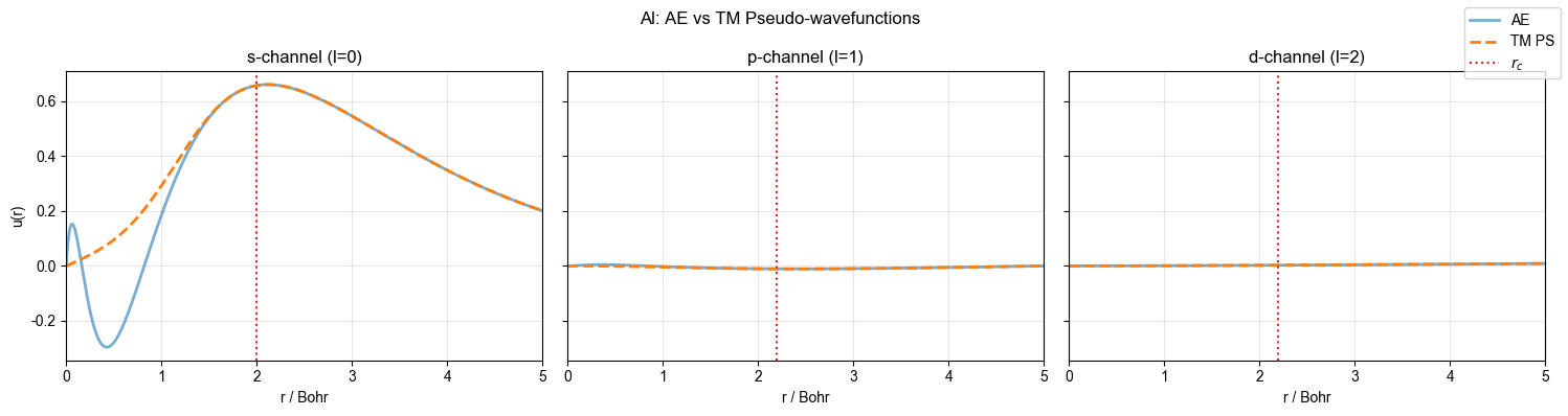
4. 可视化对比
最后,我们将全电子波函数 \(u_{\text{AE}}(r)\) 与生成的 TM 伪波函数 \(u_{\text{PS}}(r)\) 绘制在同一张图上,直观展示内区无节点特性与外区重合度。
[5]:
r = al_ae.r
fig, axes = plt.subplots(1, 3, figsize=(15, 4), sharey=True)
for ax, (l, data) in zip(axes, tm_results.items()):
    tm = data['tm']
    label_map = {0: 's', 1: 'p', 2: 'd'}

    ax.plot(r, data['u_ae'], label='AE', linewidth=2, alpha=0.6)
    ax.plot(r, tm.u_ps, '--', label='TM PS', linewidth=2)
    ax.axvline(tm.rc, color='tab:red', linestyle=':', label='$r_c$')

    ax.set_xlim(0, 5)
    ax.set_xlabel('r / Bohr')
    ax.set_title(f"{label_map[l]}-channel (l={l})")
    ax.grid(alpha=0.3)

axes[0].set_ylabel('u(r)')
handles, labels_plot = axes[0].get_legend_handles_labels()
fig.legend(handles, labels_plot, loc='upper right')
fig.suptitle('Al: AE vs TM Pseudo-wavefunctions')
plt.tight_layout()
plt.show()
小结与展望
复用 AE 求解得到的径向网格与能量,针对 s/p/d 通道构建了
continuity_orders=4的 TM 伪波函数。通过
TMResult.norm_error与eval_derivatives_at的显式比较,确认范数误差低至 \(10^{-6}\) 量级、各阶导数在 \(r_c\) 处几乎重合。可视化结果显示内外区无缝拼接,验证了所选 \(r_c\) 与网格的合理性,为后续的势反演提供了鲁棒初值。
下一讲(03-potential-inversion)将基于这些赝轨道使用 invert_semilocal_potential 提取赝势,从而完成 TM 方法的第二步:由波函数反演出局域势并做 KB 投影。欢迎继续探索。